Angular Speed and angle of a Mass on a String Lab

Purpose:

We want to find a relationship between the angular velocity (omega) of this swinging pendulum and the angle (theta) it forms as its angular speed is increased.

Experiment:

We placed a small rubber stopper at the end of a string and then gradually began to increase the angular speed of the rig shown below. Once it was moving at a constant speed, a piece of paper was placed under the spinning stopper and raised to the point of the stopper just making contact and the height was recorded. this was done for  five different angular speeds. We also recorded a period and averaged it out for each trial.

 Above is a depiction oh the equipment we were to use and the things 

to take into consideration for our calculations

Here the the the setup for the experiment. As you can see, it is very simple, a rod is attached to a motor which spins another perpendicular rod that in turn makes the rubber stopper spin around

 Here we can see Prof. Wolf (left) attempting to record the value for the height of the 

stopper and on the right we can faintly see the stopper in motion as it is 

just about to pass over the paper for a height measurement

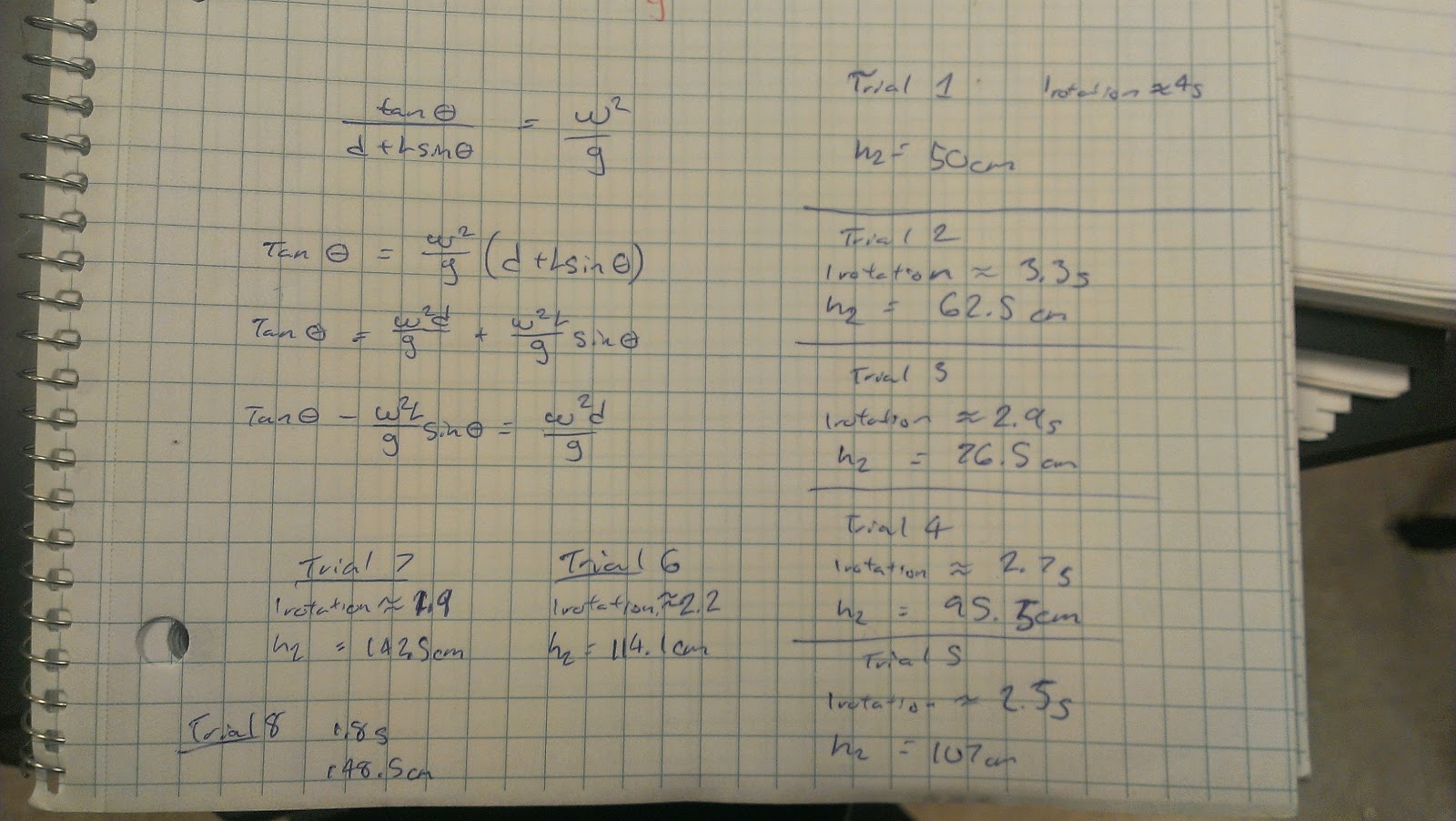
Above is our raw data that we obtained from the experiment before we calculated our theoretical relationship between the speed and angle. If you look closely, you can see that we had an equation but in order to solve for a single variable was very difficult so we just plugged it in into excel and let the program do the work for us

Here are our results with our theoretical values and actual calculated values. between the two there was only an 8% difference which is within the acceptable range considering that the way this experiment was rigged up, it had many flaws. One noticeable flaw was that the pole where the string was attached to was not level and this caused the stopper to sort of flutter in the air. Instead of traveling in a perfect circle, it had a sort of floppy motion

Finding centripetal acceleration as a function of angular speed

Purpose:
The purpose of this lab was to use an accelerometer on a turn table to show a relationship between angular acceleration and angular velocity

Experiment:
We placed a small accelerometer on the turntable and spun it at different speeds and recorded the time it took to make 4 full rotations to get an average period

Using the formula omega = 2Pi/Period we were able to input the data from the accelerometer and the period we calculated. We then used the equation a= radius*omega sqrd to solve for omega

The picture above shows a linear graph since the radius of the spinning table is constant and also shows the relationship between angular acceleration and angular velocity.

Calculating Coefficients of Static and Kinetic Friction

Purpose:

We want to calculate the Static and Kinetic frictional values for a block using different techniques

Part 1)
For the first part, we placed a block of wood on a table and attached a string to it and placed a cup on the other end. We gradually filled the cup with water until the block broke free and started to move. we recorded the mass of the cup with water and repeated this 4 times while adding a block each time.

 The picture above shows how we preformed the experiment and the data below shows what was collected of the masses of both the cup and the blocks that were used to achieve maximum static friction. We found our coefficient to be 0.260.

Part 2)
For the second part, we attached the block to a force sensor and used logger pro to record the amount of force needed to pull the block at constant speed across the same surface. This was repeated 4 times while adding a block after each trial

The two pictures above show the first and last trial where the blocks were hooked up to the force sensor and pulled at constant speed. 

Above is the data that was recorded and the coefficient friction we obtained was 0.313, which was higher than out static coefficient 

Part 3/4)

For the final two parts, we put them together and achieved only the answer to coefficient of kinetic friction. We calculated that the static coefficient at an angle would be equal to the tangent of the angle but we never actually proved this. Instead we continued on to part 4 and used a motion sensor to find the acceleration and calculate the kinetic coefficient at various angles

The picture above shows how the experiment was performed. A hanging mass that was

 just heavy enough to accelerate the block up the ramp was used and 

the motion sensor recorded the acceleration. 

 We used kinematics to solve for the kinetic coefficient of 0.234.

 Our calculated value was very similar with a value of 0.227

Conclusion:

I believe the methods we used to calculate the static coefficient on the table and incline were accurate but the methods to find the kinetic coefficient seemed to be all over the place and a reliable number could not be achieved. Especially when the block had to be pulled at a constant speed. This was difficult to replicate every time

Using Calipers and Calculating the density of Cylinders

Purpose:
In this lab we show how to calculate propagated error for each of our measurements. We will then use these measurements to calculate the density of these cylinders.

Here we have a set of calipers we used to take measurements of height and diameter in order to calculate or volume and then our density using the mass of the cylinders and the 

density formula where density = mass/ volume

Above is recorded measurements of the cylinders and the calculated density of each cylinder. 

In the lower portion of the picture you can see we used partial derivatives

 to calculate the error in each of our measurements 

After we derived a formula for calculating the uncertainty of each measurement, we plugged in our recorded values and got an uncertainty for the density of each of the cylinders 

Conclusion:

The propagated error for our results were well within an acceptable range considering that our scale and calipers had an error of ± 0.1. For this experiment, it was well within the accepted values.

Projectile Motion Lab

Purpose: 

The purpose of this lab is to calculate a balls initial horizontal velocity as it leaves an aluminum channel and predict where it will land on a horizontal surface as well as an inclined surface.

Procedure:

We setup an aluminum channel to guide a steel ball down the ramp and into a horizontal channel to then launch it off a table. We placed a piece of carbon paper on the floor and recorded where the ball landed . We then measured the distance the ball traveled away from the table and the height of the table. We then used kinematics to find out initial velocity the ball left the table

Here are two pictures of our setup with the carbon paper placed on the 

floor in front of the edge of the table

A short video of our experiment where we allowed the ball to land on the floor

Here we repeated the same experiment but only this time the ball was made to land on an angled surface. After the angle was recorded, we setup some kinematics equations to determine how far down the plank the steel ball would land

In the picture above, we calculated the initial horizontal velocity of our steel ball. First we symbolically solved for time and then plugged in this equation into our horizontal component equation to calculate our initial velocity. From our recorded data we measured the 

height from table to floor as 0.938 m and the Horizontal distance as 0.835 m. 

This gave us an initial horizontal velocity of 1.909 m/s

Here we measured the angle of our plank as 36 degrees. From this, we derived a formula to calculate the distance d that the ball would hit on the plank. Using our initial velocity of 1.909m/s and angle of 36 degrees, we got an answer of d =0.667 m or 0.67 m down the plank from the edge of the table. After the theoretical calculation was made, we performed 5 trials and were able to match our  distance with a recorded experimental value of d= 0.68 m.

Conclusion:

Overall, the lab was a success and we were able to match our predicted result with our experimental result. The only uncertainty we could factor in was the height from where the ball was dropped from might have been slightly different each time but we later fixed this by setting a common dropping point with a piece of tape to ensure consistent data

Modeling Free Fall with coffee filters Lab

The purpose of our lab was to find relationship between air resistance force and speed. We will find the relationship by dropping coffee filters. By graphing the data we collect we can use it to find a power fit for the air resistance formula F-resistance = kv^n. After we graphed our data and found the values for k and n, we used Excel to  compare our experimental graphs to our modeled graphs.

Data Collection

For this experiment, we used a camera to capture the motion of the coffee filters as they fell a one story inside the design technology building. We started off with only one filter and repeated this five times. For each trial one filter was added until we had a total of five filters. We also used a two meter stick as a reference so logger pro could estimate the total distance the filter had fallen. After setting the reference, we could then determine the terminal velocity for each of the trials

The video above shows a similar example of the procedure performed to recorded the position of the coffee filters.

In this picture we show the terminal velocity for each trial starting with one filter on the bottom left and continuing clockwise. As you can see, our terminal velocity for each trial is increasing as the mass of filters increases thus proving that the upward force on the filters is being overcome by the added mass.

Here is a graph of the force versus velocity which yielded us with

a k value of 0.0055 and n value of 1.9247.

With our experimental data now collected, we used the  k and n values to make a model of a falling filter with air resistance by using Excel  and using a time interval of 1/30 of a second. 

Conclusion

Our data is only as good as our equipment and using an outdated camera that can not record very clearly is not a good start.  The  data is decent for all the graphs and are very similar when comparing their slopes. Overall I think the experiment went great even though we were not able to replicate our models to look similar to the data we recorded.

Sparker Free Fall Lab

Purpose: In this lab, we will show the motion of a free falling mass to determine the value for gravity. The device shown in the picture below will cause a spark to mark a piece of paper at an interval  of 1/60th of a second until it travels a distance of approximately 1.5m. One we have our data, we will be able to plot a position vs time graph and be able to calculate the acceleration of the mass.

In the image below, we have our paper strip line up with our meter stick in order to gather our data. Here we can observe that the small marks on the paper are getting further and further apart as we go down the strip, indicating the mass was accelerating.

Below is our data that we input into excel to calculate or mid-interval times and speeds. When plotted , the slope of the line will be our experimental acceleration. Note that the mid-interval speeds are in cm/s and not in m/s.

Here is the plotted data and our slope reveals and acceleration value of roughly 9.7 m/s/s. This shows that our experimental value for gravity was 1% off of the accepted value of 9.8 m/s/s.

Conclusion: Our experiment showed that the value of g was very close to the accepted value of g and was only 1% off. By using our data and plotting it with a trend line in excel, we were able to show the acceleration of the falling mass. We could have also found this by plotting our position and time graph and finding an equation for this time. From there we could have derived a formula for position and then calculated a formula for velocity.

PHYS 4A Non-Constant acceleration Activity

Purpose: In this lab we are depict a 5000 Kg elephant with a rocket strapped to its back and try to determine how far the elephant goes before it stops. The rocket provides a constant 8000 N Force and burns fuel at a rate of 20 kg/s so it mass changes according to the following equation m(t) = 1500-20t.

We start off with or acceleration function

 After we integrate the acceleration function, we get our velocity function below
 And finally, we integrate for a third time and we get our position function below.

The data set below depicts all three functions. The highlighted portions on both spread sheets represent the time, distance and velocity of the elephant when it changes direction of motion. The picture below shows a time interval of 0.05 seconds difference and we show a total horizontal distance of 248.67m

The image below is similar but shows a time interval change of .10 seconds. Horizontal distance remains the same as well as the time elapsed to slow down and change direction

Conclusion: After we solved for all the functions and used Excel to plot our data, we showed that the time needed to stop the elephant was 19.69 s and the distance the elephant had traveled equated to 248.7 m. We were able to get very precise with our numbers by changing the time interval to different amounts and finding where out velocity would be equal to 0. In our case, it turns out to be around 19.6 seconds. We chose these intervals because they gave us the closest amout to 0 as we could get without getting to extreme on our precision.

Deriving a Power law for an inertial pendulum

Over the course of two class periods, we were tasked with the challenge to find a relationship between mass and period using an inertial balance. Since a spring scale and balance use gravity to find mass, if no gravity is present, they would be useless to find an unknown mass. For this reason, we use and inertial balance to find the mass of the object by measuring the balance's resistance to change in motion.

Here is a picture of the setup of the inertial balance with 800g of mass added and the equipment recording the data from the oscillations of the balance.

PROCEDURE

A C-clamp was used to secure the balance to the table and a piece of tape was used to break the beam between the photgate. After the computer was setup, measurements of the period of the balance with different masses were taken and recorded. We started with just the balance and added 100g after each measurement until we reached our maximum mass of 800g. Below is a table of our data. As you can see, the more mass that is added, the slower the period is.

After we recorded our data, we used 2 different objects(in our case a cell phone and water bottle) and placed them on the balance and recorded their periods. We will use these periods to determine if our power law equation is accurate or not.

THE POWER-LAW EQUATION

We now have to find a relationship between mass and period using a power equation. We started off by using the base equation below and reworked it to mimick the form of an equation of the line.

 We then plotted out data into a mass v. period graph in logger pro and used a line fir to provide us with our constants of the mass of the tray. We found a range of the mass of the tray which yielded us with a 0.9999 correlation between the graph and our points. We then used this range to best provide our team with a mass of our objects.

Here is the final equation which will give us our mass of our known objects of varying mass

At first, our numbers were not matching up but we then realized that we had to use an exponential in the base of the exponential and this solved our problem. The final result was an equation that yielded us an answer that was within ± .001g of the actual maass. Needless to say, this equation was very accurate.