Two Dimensional Collisions

Purpose:
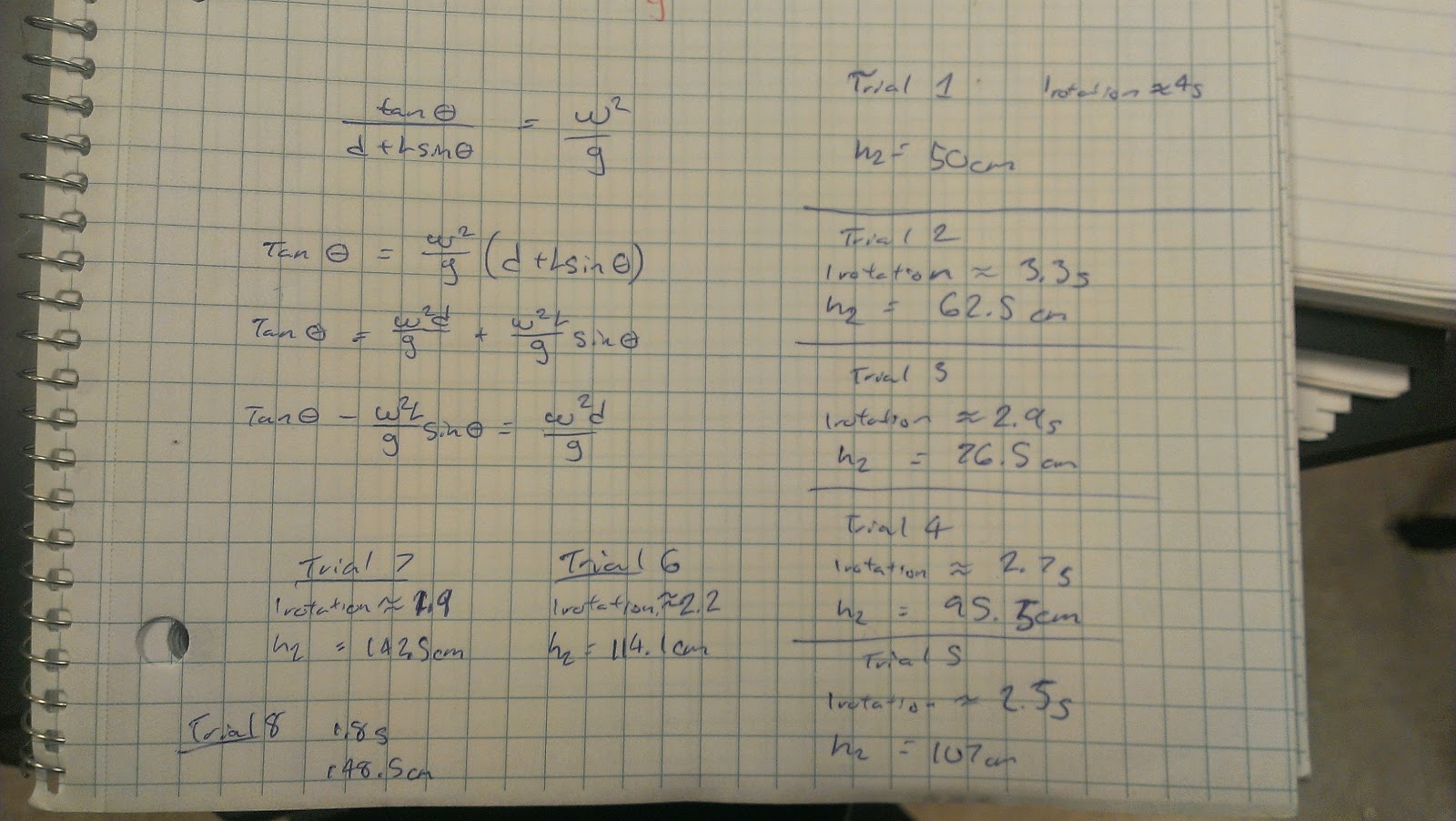
The purpose if this lab is to look at the collisions between two steel balls and between a marble and steel ball to see if momentum is conserved in both cases

Experiment:
We will be using a level table with a camera set up above to capture the motion of the two collisions mentioned above. Here is our setup.

 Here are the videos of the two collisions
The first shows the two marbles
The second shows the marble and the steel ball

After we performed these collisions, we used logger pro to plot the paths of each collision to find our momentum before and after the collisions. Using those graphs, we could then plot the momentum of each and show whether it was conserved or not as well as the kinetic energy of each

Unfortunately after all that work, i was unable to find the graphs of the positions of the collisions so i will skip ahead to the momentum's of each collision

Marble vs Marble Collision:

The green tick marks represent Total Kinetic Energy

The light blue triangles represent momentum in the Y directions

The blue squares represent momentum in the X direction

Although the graph doesn't show a straight lie for kinetic energy, 

it was conserved and it relatively straight

Marble vs Steel Ball:

The green diamonds marks represent Total Kinetic Energy

The light blue triangles represent momentum in the Y directions

The green crosses represent momentum in the X direction

Same as above, Kinetic energy is conserved even the the graph shows otherwise

Although our videos and our analyzation of the video wasn't very accurate, our team was satisfied with the results. we could have gotten better data if the marbles were bigger and we had better video capture

Impulse and Momentum

Purpose:

In this lab we are trying to find the impulse that was exerted onto the cart as a result of an elastic collision. Since the impulse is the change in momentum, we can use the force exerted during the collision and the velocity before and after to calculate this

Experiment:

 We will be using two carts to for this experiment. In the first part we held one cart on a pole, while the other cart was fitted with a force sensor and given a push towards the other cart where they would collide elastically. Below is a picture of the setup from the POV of the motion sensor.

Here is the graph of the data that was collected for the force, position and time. The middle graph shows the carts position as it approaches and then collides with the other cart. The top graph shows the force exerted by the cart. If we integrate this graph, we can find the momentum of the cart during the collision which was -0.4053 N/s. We got a negative value because we did not reverse the direction of the position sensor but in our own calculation we got a value of -0.397N/s

The next part of this lab, we had a volunteer who was willing take a few hits from the cart with a force sensor in the spirit of physics. So this time, instead of an elastic collision, we will have a totally inelastic collision. We will be recording the same data as before.

Here is a graph of our data which shows the cart did not return after the collision. Since the cart doesn't return, momentum is not conserved and the full brunt of the force is taken by our brave volunteer. Momentum for the collision was recorded to be -0.3136 N/s

Magnetic Potential Energy

Purpose:

For this lab, we are trying to find a relationship between a magnet and its potential energy, which does not fit Hooke's law for a spring.  In order to calculate this, we need to measure force vs. separation distance.

Experiment:

For the first part, we will be using an air track with a cart to make a near friction-less surface for the cart to glide upon. This will ensure we record accurate measurements and the separation distance is not influenced by friction. We also attach magnets to one end of the cart and on the other end of the track which were set to repel each other. Below is a picture of the setup with the cart and air pump.

In order to get data points for a graph, we had to create a greater force on the cart. We used large physics books to elevate one end of the track to various angles and decrease the separation distance, thus giving us different distances. We also used an equation to calculate the force of the cart

Force = mgh * Cos(x), where x is the measured angle

Once we had out data points, we could plot them on a graph and let Logger Pro calculate a power fit for us which would give us values for A and B. Using these values we could establish an equation for the potential energy of the magnets we were using.

Now that we have our equation for the potential energy of the magnets, we leveled the track and used a motion sensor to track the position and velocity of the cart as we pushed it towards the end of the track where the other magnets were.

We then made a graph to show the potential, kinetic and total energy in the system.

The final graphs show position vs time in the top and total energy on the bottom
The red line shows total energy, which was conserved, while the purple shows potential energy of the magnet and the orange shows kinetic energy of the cart

Conservation of Energy with an Oscillating Mass on a Spring

Purpose: In this lab we show the the conservation of energy in a system consisting of a mass hanging on a spring. To do this we will need to measure the kinetic energy of the mass, kinetic energy of the spring, potential energy of the mass, potential energy of the spring, the elastic energy in the spring, gravitational potential energy of the spring, and finally the total of all the energies listed above.


Experiment: For this we need a spring with a mass attached to one end and fixed to another point. We place a sensor below the mass to capture the motion of the mass-spring system. We first have to calculate a spring constant to use in our equations. We used mg=kx where m is the mass of the spring and x is the displacement of the spring.

We first had to calculate the individual energies within the system which would give us the total energy. As you can see in the pictures above and below, we found the PE, KE and  SpringPE

In the picture above, we have the total energy in the system which can be shown in 5 different equtions: KE of the mass, PE of the mass, Elastic PE of the Spring, KE of the spring and the GPE of the spring. Position data from the experiment would be used to calculate GPE and Elastic PE while velociity would be used to calculate the KE in the system

 

Above we have a picture of our setup using a spring and a mass hanging from the end. We places a motion sensor at the bottom to record the motion of the mass and get our data chart below

Here we have the data that was collected and placed all together on this graph. as you can see, the total energy in the system was conserved, thus proving our theory that all energy is conserved in this system. the different colored lines each represent a type of energy and go as follows
Orange: Total Energy in system
Purple: Potential Energy of the mass
Red: Elastic Potential energy of the Spring
Green: Potential Energy of the Spring
Yellow/Orange: Kinetic Energy of mass
Blue: Kinetic Energy of the spring

Work-Kinetic Energy Theorem Lab

Purpose:

For this lab, we are trying to prove the Work-KE theorem which states that the integral of the force with respect to position (work) is equal to the Kinetic Energy at the same point in position.

Experiment:
We place a cart with mass m and connect it to a spring which is then connected to a force sensor. On the opposite end, we have a motion sensor that detects the position of the cart. We set the equilibrium point of the cart as our initial position x=0 and pull the card back a small distance. We then let go of the cart and record the data.

Above is a picture of our cart being pulled 

Above we have the force exerted by the spring in the Purple line. The red shading represents the integration of force which matched our selected points on the graph 

Angular Speed and angle of a Mass on a String Lab

Purpose:

We want to find a relationship between the angular velocity (omega) of this swinging pendulum and the angle (theta) it forms as its angular speed is increased.

Experiment:

We placed a small rubber stopper at the end of a string and then gradually began to increase the angular speed of the rig shown below. Once it was moving at a constant speed, a piece of paper was placed under the spinning stopper and raised to the point of the stopper just making contact and the height was recorded. this was done for  five different angular speeds. We also recorded a period and averaged it out for each trial.

 Above is a depiction oh the equipment we were to use and the things 

to take into consideration for our calculations

Here the the the setup for the experiment. As you can see, it is very simple, a rod is attached to a motor which spins another perpendicular rod that in turn makes the rubber stopper spin around

 Here we can see Prof. Wolf (left) attempting to record the value for the height of the 

stopper and on the right we can faintly see the stopper in motion as it is 

just about to pass over the paper for a height measurement

Above is our raw data that we obtained from the experiment before we calculated our theoretical relationship between the speed and angle. If you look closely, you can see that we had an equation but in order to solve for a single variable was very difficult so we just plugged it in into excel and let the program do the work for us

Here are our results with our theoretical values and actual calculated values. between the two there was only an 8% difference which is within the acceptable range considering that the way this experiment was rigged up, it had many flaws. One noticeable flaw was that the pole where the string was attached to was not level and this caused the stopper to sort of flutter in the air. Instead of traveling in a perfect circle, it had a sort of floppy motion

Finding centripetal acceleration as a function of angular speed

Purpose:
The purpose of this lab was to use an accelerometer on a turn table to show a relationship between angular acceleration and angular velocity

Experiment:
We placed a small accelerometer on the turntable and spun it at different speeds and recorded the time it took to make 4 full rotations to get an average period

Using the formula omega = 2Pi/Period we were able to input the data from the accelerometer and the period we calculated. We then used the equation a= radius*omega sqrd to solve for omega

The picture above shows a linear graph since the radius of the spinning table is constant and also shows the relationship between angular acceleration and angular velocity.